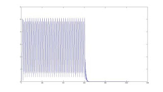
This a program in MATLAB. This program shows you, how the digital filter filters a desired frequency from an input signal.
I had written two methods for doing this.One methods is using Convolution (filtering takes place in time domain)and the other is using the property of convolution (filtering action takes place in frequency domain). In this program the input signal is selected such that it contains two frequencies and both are present all the time. Since this is a Linear time invariant signal we can do the filtering in frequency domain too.
The basic algorithm of this program is as follows:
1) sample the input signal
2) plot the signal, its sampled version, and its frequency components
3) finding the FFT
4) Plot it .
5) designing a low pass filter
6) displaying filter response
7) In Frequency domain method
a) multiply both responses
b) displaying the resultant response
c) finding inverse fft
d) displaying it;
In Time domain method
a) finding the impulse response of filter
b) convoluting it with input signal
c) displaying it.
8) END
DOWNLOAD
Program using Convolution
%% filtering of an input signal using convolution
% vipin.p.nair
% 28-sept-2009
%% observations
% 1) when we increse the signal duration the power
% content will also increase.
% 2) anplitude of power also increases with increase
% of N
% 3) we need to display only the the frequency up to FS/2
% bcz the values beyond it will be a mirror image of the
% first. ie we are displaying 0 to pi.
%% program
clear all
f1 = 2000;
f2 = 1000;
t=.002; % input signal duration in seconds.
Ts = 1/50000;
n = 0: Ts :10*t;
x = 5*sin(2*pi*f2*n) + 5*cos(2*pi*f1*n);
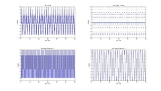
figure(1);
subplot(2,2,1), plot(n*1000, x);
title 'Input signal';
xlabel 'time (ms)'
ylabel 'voltage'
grid;
subplot(2,2,2), plot(n*1000, x, '.');
title 'Input signal samples';
xlabel 'time (ms)'
ylabel 'voltage';
grid;
subplot(2,2,3), plot(n*1000,5*cos(2*pi*f1*n));
title 'Input signal frequency -1';
xlabel 'time (ms)'
ylabel 'voltage'
grid;
subplot(2,2,4), plot(n*1000,5*sin(2*pi*f2*n));
title 'Input signal frequency -2';
xlabel 'time (ms)'
ylabel 'voltage'
grid;
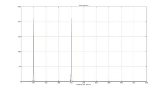
% frequency spectrum of input signal
N =1024*1;
Xk = fft(x,N);
Pxx = Xk .* conj(Xk)/N;
figure(2);
plot((0:N/2)/(N*Ts),(Pxx(1:N/2+1)));
title 'Power spectrum'
xlabel 'Frequency (Hz) upto Fs/2'
grid;
% filter
filter_order = 10;
Fs = 1/Ts;
fc = 1500 / ( Fs/2) ;
[b,a] = butter(filter_order, fc);
w = 0: 2*pi/(N-1) :pi;
[H,wn2] = freqz(b,a,w);
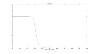
figure(3)
plot(w/pi*Fs/2,(abs(H)));
h = ifft(H,length(n));
out = cconv(abs(h),x);
ln=length(n);
figure(4);
plot(n*1000,out(1:ln));grid;
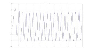
title 'Signal after filtering'
OUTPUT FIGURES
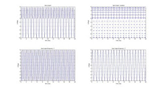
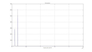
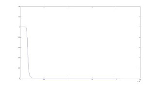
Program using filtering in frequency domain
%% filter
% vipin.p.nair
% sept- 28- 2009
% observations
% 1) when we increse the signal duration the power
% content will also increase.
% 2) anplitude of power also increases with increase
% of N
% 3) we need to display only the the frequency up to FS/2
% bcz the values beyond it will be a mirror image of the % first. ie we are displaying 0 to pi.
clear all
f1 = 2000;
f2 = 500;
t=0.06; % input signal duration in seconds.
Ts = 1/10000;
n = 0: Ts :t;
x = 5*sin(2*pi*f2*n) + 5*cos(2*pi*f1*n);
figure(1);
subplot(2,2,1), plot(n*1000, x);
title 'Input signal';
xlabel 'time (ms)'
ylabel 'voltage'
grid;
subplot(2,2,2), plot(n*1000, x, '.');
title 'Input signal samples';
xlabel 'time (ms)'
ylabel 'voltage';
grid;
subplot(2,2,3), plot(n*1000,5*cos(2*pi*f1*n));
title 'Input signal frequency -1';
xlabel 'time (ms)'
ylabel 'voltage'
grid;
subplot(2,2,4), plot(n*1000,5*sin(2*pi*f2*n));
title 'Input signal frequency -2';
xlabel 'time (ms)'
ylabel 'voltage'
grid;
% frequency spectrum of input signal
N =1024*1;
Xk = fft(x,N);
Pxx = Xk .* conj(Xk)/N;
figure(2);
plot((0:N/2)/(N*Ts),(Pxx(1:N/2+1)));
title 'Power spectrum'
xlabel 'Frequency (Hz) upto Fs/2'
grid;
% filter
filter_order = 10;
Fs = 1/Ts;
fc = 1500 / ( Fs/2) ;
[b,a] = butter(filter_order, fc);
%'syms z
%v=tf (b,a);
w = 0: 2*pi/(N-1) :pi;
[h,wn] = freqz(b,a,w);
[h2,wn2] = freqz(b,a,0: 2*pi/(N-1): 2*pi);
figure(3)
plot(wn/pi*Fs/2,(abs(h)));
title 'Filter response'
xlabel 'Frequency (Hz) upto Fs/2'
figure(4)
Yk = h.*Xk(1:N/2);
Yk2 = h2.*Xk;
plot(wn/pi*Fs/2,(abs(Yk)));
xlabel 'Frequency (Hz) upto Fs/2'
title ' frequency spectrum after filtering'
grid;
%figure(5)
%plot(wn/pi*Fs/2,(abs(Xk(1:N/2))));
%grid;
figure(6)
plot(abs(ifft(Yk2,N)));
OUTPUT:
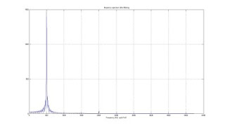
Output signal waveform
