Problem:
Here is an attempt to solve a simple R-L-C circuit using space vector representation using MATLAB. In this post we will see discuss on
1. Constructing State Space representation
2. Plot the output voltage across capacitor using MATLAB 'ss' commands
3. Plot same without using state space function (ss) in MATLAB.
Introduction:
Most of the undergraduate students would be familiar with constructing either differential equations or Laplace equations of an RLC circuit and analyse the circuit behavior. But apart from this classical methods one could use State space matrices also to solve this kinds of problems, which is widely used in modern control systems.
State space representation of a given system helps to solve differential equations of any order to simple linear differential equations of first order. The state of the system shall be found out in time domain itself rather than going to frequency domain and solving it. Another advantage of using this method is initial value of energy storing elements such as capacitors (voltage) and inductors(current) shall easily be considered, once state equations are available. This make it differs from Laplace equations where we consider initial conditions of the energy storing elements as zero though its possible to make Laplace equation of system considering the initial conditions.
Figure1: RLC circuit

Consider figure 1 which shows an RLC circuit. Here R, L and C are in series. Practically one could consider it as a part of Buck Converter or shall be considered as Low side MOSFET driving an inductive load with coil resistance R and ESD capacitor or Coss of MOSFET as C in circuit. RL is representing the load resistance. Consideration of load resistance will help to consider the loading effect experienced by the circuit, helps to get output close to practical scenario.
Making of State space representation
This has two parts. One is state equation and another is output equation.
ẋ = Ax + Bu --------------> State equation
y = Cx + Du --------------> Output equation
ẋ = First derivative of state vector matrix 'x'
u = Input to the system. (It is represented as Vg also )
y = Output matrix
A = Evaluation matrix
B = Control Matrix
C = Observing Matrix
D = Transition Matrix
This shall be represented in below form also. This is what considered in method-2 matlab program. This will be discussed later.
Fig2:

or

Now we shall consider constructing these matrices. Vc and IL are considered as state vectors. Consider KVL & KCL and form following equations
Vo = Vc
 Note: Edited on 2nd may for typo errors.
So above differential equations shall be represented in below matrix form
for state equation (ẋ = Ax + Bu ):

and for output equation (y = Cx + Du)

dot(iL) = d(iL)/dt
dot(Vc) = d(Vc)/dt
---------------------------------------------------------------------------------------
So its time to plot the output curve
Method 1:
This is the standard method which one shall follow in MATLAB.
% RLC circuit
% 30/04/2014
% author: vipin p nair
R = 0.1;
C = 330e-6;
L = 22e-6;
RL=10e+3;
% State variables
A_SS = [-R/L -1/L ; 1/C -1/(C*RL)];
B_SS = [1/L; 0];
C_SS = [0 1];
D_SS = [0];
% state vectors
% edited 2nd may
% initial conditions iL & Vc are zero initially
% command 'initial' shall be used to plot with initial condition'
G = ss(A_SS, B_SS, C_SS, D_SS);
impulse(G);
figure;
step(G);
% edited: 2nd May
% plot with initial condition
initial(G, [iL ; Vc]);
[y, t, x]=initial(G, [iL ; Vc]); % to take values with out plotting
Output:


Method 2 : By considering fig2 and plotting same output without using ss function.
considers integration using summation inside the 'for' loop
% RLC circuit
% 30/04/2014
% author: vipin p nair
clear all;
R = 0.1;
C = 330e-6;
L = 22e-6;
RL=10e+3;
% State variables
A_SS = [-R/L -1/L ; 1/C -1/(C*RL)];
B_SS = [1/L; 0];
C_SS = [0 1];
D_SS = [0];
% state vectors
% initial conditions
iL = 0;
Vc = 0;
xout = [iL; Vc];
% initial condition
u = 1; % 1volt step input
Bu = B_SS.*u;
xbar_array = [0; 0];
xout_array = [0; 0];
for i=1:3000
Ax = A_SS*xout;
xbar = Bu + Ax;
xbar_array = [xbar_array, xbar];
% considers 1us as delta T for integration
xout = transpose(sum(transpose(xbar_array))).*0.000001;
xout_array = [xout_array, xout];
end
y = transpose(xout_array);
plot(y(1:3000,2));
xlabel 'time in microseconds';
ylabel 'Amplitude';
title 'Step response'
Output:

Hope this article is clear. Try it out!!! Comment your doubts.
1. Constructing State Space representation
2. Plot the output voltage across capacitor using MATLAB 'ss' commands
3. Plot same without using state space function (ss) in MATLAB.
Introduction:
Most of the undergraduate students would be familiar with constructing either differential equations or Laplace equations of an RLC circuit and analyse the circuit behavior. But apart from this classical methods one could use State space matrices also to solve this kinds of problems, which is widely used in modern control systems.
State space representation of a given system helps to solve differential equations of any order to simple linear differential equations of first order. The state of the system shall be found out in time domain itself rather than going to frequency domain and solving it. Another advantage of using this method is initial value of energy storing elements such as capacitors (voltage) and inductors(current) shall easily be considered, once state equations are available. This make it differs from Laplace equations where we consider initial conditions of the energy storing elements as zero though its possible to make Laplace equation of system considering the initial conditions.
Figure1: RLC circuit
Consider figure 1 which shows an RLC circuit. Here R, L and C are in series. Practically one could consider it as a part of Buck Converter or shall be considered as Low side MOSFET driving an inductive load with coil resistance R and ESD capacitor or Coss of MOSFET as C in circuit. RL is representing the load resistance. Consideration of load resistance will help to consider the loading effect experienced by the circuit, helps to get output close to practical scenario.
Making of State space representation
This has two parts. One is state equation and another is output equation.
ẋ = Ax + Bu --------------> State equation
y = Cx + Du --------------> Output equation
ẋ = First derivative of state vector matrix 'x'
u = Input to the system. (It is represented as Vg also )
y = Output matrix
A = Evaluation matrix
B = Control Matrix
C = Observing Matrix
D = Transition Matrix
This shall be represented in below form also. This is what considered in method-2 matlab program. This will be discussed later.
Fig2:
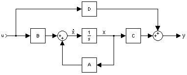
From Wikipedia
or
Now we shall consider constructing these matrices. Vc and IL are considered as state vectors. Consider KVL & KCL and form following equations
Vo = Vc
for state equation (ẋ = Ax + Bu ):
dot(iL) = d(iL)/dt
dot(Vc) = d(Vc)/dt
---------------------------------------------------------------------------------------
So its time to plot the output curve
Method 1:
This is the standard method which one shall follow in MATLAB.
% RLC circuit
% 30/04/2014
% author: vipin p nair
R = 0.1;
C = 330e-6;
L = 22e-6;
RL=10e+3;
% State variables
A_SS = [-R/L -1/L ; 1/C -1/(C*RL)];
B_SS = [1/L; 0];
C_SS = [0 1];
D_SS = [0];
% state vectors
% edited 2nd may
% initial conditions iL & Vc are zero initially
% command 'initial' shall be used to plot with initial condition'
G = ss(A_SS, B_SS, C_SS, D_SS);
impulse(G);
figure;
step(G);
% edited: 2nd May
% plot with initial condition
initial(G, [iL ; Vc]);
[y, t, x]=initial(G, [iL ; Vc]); % to take values with out plotting
Output:
Method 2 : By considering fig2 and plotting same output without using ss function.
considers integration using summation inside the 'for' loop
% RLC circuit
% 30/04/2014
% author: vipin p nair
clear all;
R = 0.1;
C = 330e-6;
L = 22e-6;
RL=10e+3;
% State variables
A_SS = [-R/L -1/L ; 1/C -1/(C*RL)];
B_SS = [1/L; 0];
C_SS = [0 1];
D_SS = [0];
% state vectors
% initial conditions
iL = 0;
Vc = 0;
xout = [iL; Vc];
% initial condition
u = 1; % 1volt step input
Bu = B_SS.*u;
xbar_array = [0; 0];
xout_array = [0; 0];
for i=1:3000
Ax = A_SS*xout;
xbar = Bu + Ax;
xbar_array = [xbar_array, xbar];
% considers 1us as delta T for integration
xout = transpose(sum(transpose(xbar_array))).*0.000001;
xout_array = [xout_array, xout];
end
y = transpose(xout_array);
plot(y(1:3000,2));
xlabel 'time in microseconds';
ylabel 'Amplitude';
title 'Step response'
Hope this article is clear. Try it out!!! Comment your doubts.
it can be less curvy n STRAIGHT.
ReplyDeleteThank you so much
ReplyDelete